Step Function Regression for 1D Data And Grid Search

Let's consider the following supervised learning problem. We have data with a single coordinate and two classes we want to sort it into: blue dots (0) or orange stars (1), as shown below:

For our model, let's try to create a function of a single variable x that returns a 0 for some ranges of x where we find the blue dots, and a 1 for other ranges of x where we find the orange dots. The simplest possible function we could define is a step function

In other words, we want to find a single threshold a above which we believe we have an orange star, and below which we've decided we have a blue dot. We shouldn't expect to get this 100% correct on the above example since they're mixed together a bit, but this is not a bad model since most of the orange stars are to the right of most of the blue dots.

To score how well different a values work across all of our data points (x_i, y_i) (where y_i is the label, either 0 or 1, that x_i has), we can use a squared loss loss function which is the sum of the squared distances between f_a(x_i) and the true values of the dots. This loss would look like this

In the case of the step function on the above data, this means we add a penalty of 1 for every point that is misclassified. If we think back to calc 1, the way that we usually minimize functions is by finding critical points. Most of the critical points are found by setting the derivative equal to 0 and solving. The problem with the step function, though, is that it's non-differentiable, so this becomes a pain. We can instead use something called grid search where we try a whole bunch of values evenly spaced over an interval and see which one leads to a min (an even smarter thing to do in 1D is to use golden section search). Here's some code that does grid search with 1000 points over the interval [-1, 8]

If we do this on the above example and plot the loss function at each a we try, we get this:

There are a few global mins at a loss of 6, one of which occurs at around a = 2.7. As shown below, if we plot the value of the step function versus the ground truth value of our data (class 0 or class 1), we can see that 3 orange points got misclassified and 3 blue points got misclassified.

This seems like it worked out pretty well! The problem is that it doesn't scale if we're trying to fit a model that has more than one parameter. For example, if we have two parameters and we likewise divvy up the range into 1000 evenly spaced regions for each parameter, we have to try a million parameter combinations. If we have 3 parameters, we have to try a billion. And in general, if we take N samples of each parameter and we have P parameters, we will have to try N^P parameter combinations! This is known as the curse of dimensionality. To give you an idea of how bad this is, when we go to classify images, we will have on parameter for pixel. In a fairly small 100x100 image, this is 10,000 pixels. If we try even a paltry 10 unique parameter values in grid search, we get 10^10,000 different combinations, which is beyond astronomical. We're definitely going to need a more sophisticated technique.

---

1D Logistic Regression

Let's now try to come up with something that acts like the step function but which is differentiable. We'll use something called the logistic function, which is defined as

If you plot it, you'll see it's like a step function that makes a smooth transition from 0 to 1

This means it acts like the function we were looking for that chooses a boundary between the objects in class 0 and class 1, but it's differentiable. If we use the chain rule, we can compute its derivative as

Actually, there's a really slick way to rewrite this as just the following (which you can check with some algebraic manipulations)

Now let's think about how we might fit the logistic function to our data. Actually, we'll allow ourselves to have two parameters now: one called a which controls the sharpness of the increase from 0 to 1, and one called b which controls a horizontal shift (at this point you may want to stop and review how to stretch out and horizontally shift functions). In particular, we'll consider how the equation

best fits our data. Then we can define our squared loss loss function as follows

We want to minimize this function. As an example of what this looks like, let's fix a = 1 and look at grid search again over the horizontal shift parameter b

But let's see what we can do towards optimizing both parameters jointly with a more sophisticated technique. In class, we saw how instead of doing a full on grid search, we could look in a small neighborhood around each point and walk in the direction of where the function seems to be decreasing, and then to repeat this process. One fundamental optimization technique for doing mathematically is gradient descent, whereby we compute the derivative of our loss with respect to each parameter, treating everything else as a constant. This is referred to as the partial derivative ∂ with respect to each parameter. For example, let's consider the partial derivative of our loss with respect to the parameter a. We can obtain this with multiple applications of the chain rule, noting that everything other than a is a constant

By a similar procedure, we find that the partial derivative with respect to b is

Since the derivative tells us how the function is increasing, we want to walk along the opposite direction. Therefore, we will update our parameters a and b by subtracting some nonnegative constant μ times the derivative. This parameter μ is sometimes referred to as the learning rate

Here's what gradient descent looks like after modifying the starter code here, with a step μ = 0.1

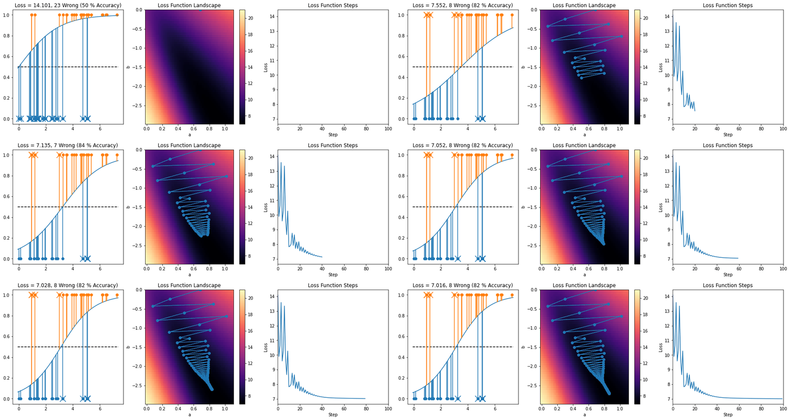
This step size is a bit large and causes it to zig zag. Here is a smaller step size μ = 0.01, which moves more slowly but which does not cause the same zig zagging:

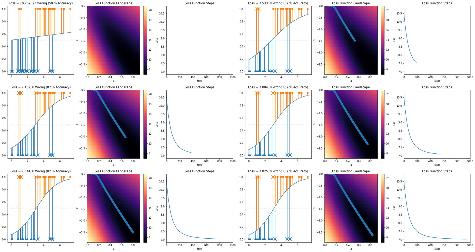
We should be mindful of this tradeoff as we choose our learning rate.

---

Separating Lines in 2D / Higher Dimensional Logistic Regression

We can extend these ideas to higher dimensions. The very next dimension up leads us to a procedure for separating lines in 2D. Here, the boundary decision boundary is described with the equation ax + by + c = 0, so there are three parameters: a, b, and c. Let's now suppose the class labels of our planar data points (x_i, y_i) are called z_i to avoid a variable name collision. This leads us towards minimizing the loss function

We can work through similar math to find the following update rules for gradient descent

where

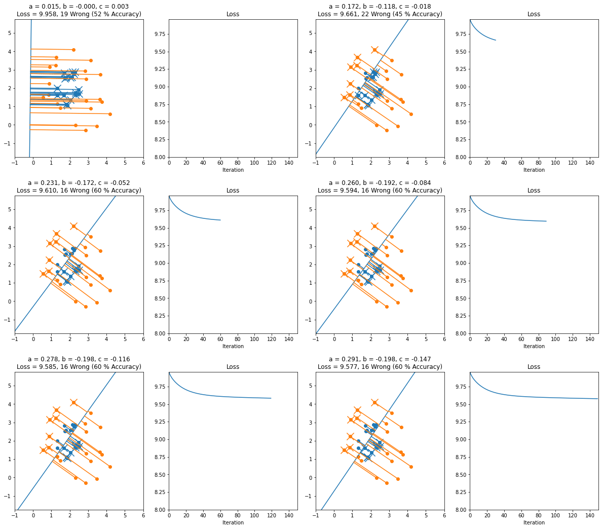
Here's an example of a working implementation of gradient descent on 2D data starting from this file

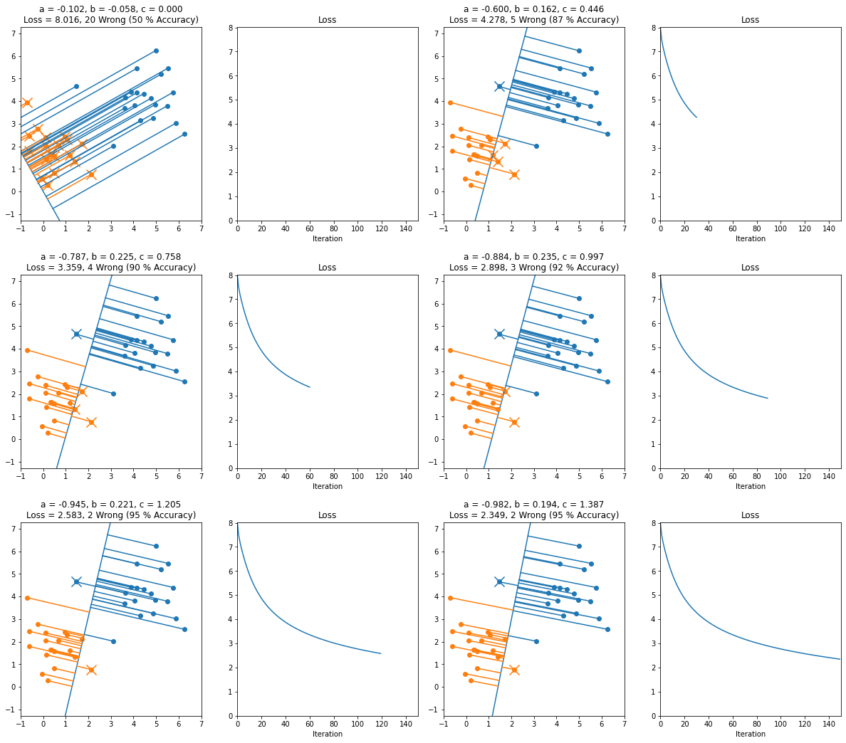
Here's another example where the line started off in the backwards orientation

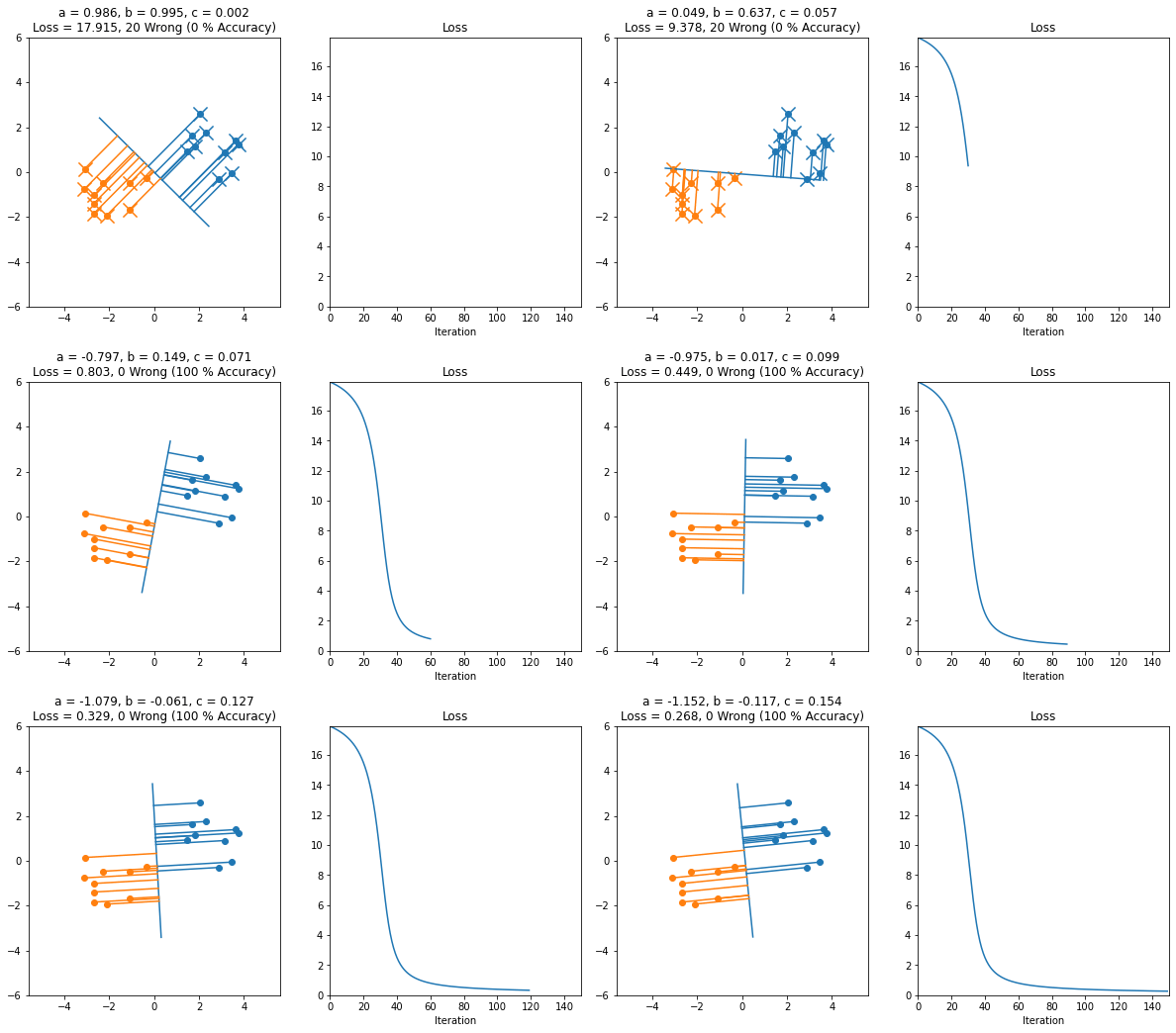
Here's an example where the data isn't separable

Higher Dimensions

In general, we can run logistic regression on d independent variables x₁, x₂, ... x_d by fitting with the logistic function composed with

In that case, we can update all of the w's as

\[ \frac{\partial L(w_1, w_2, ..., w_d, c)}{\partial w_k} = \sum_{i=1}^N 2 x_k( f(\vec{w}, c) - z_i) f(\vec{w}, c)(1-f(\vec{w}, c)) \]

\[ \frac{\partial L(w_1, w_2, ..., w_d, c)}{\partial c} = \sum_{i=1}^N 2 ( f(\vec{w}, c) - z_i) f(\vec{w}, c)(1-f(\vec{w}, c)) \]

where w with an arrow over it represents a vector of all ws

\[ f(\vec{w}, c) = f( w_1x_1 + w_2x_2 + ... + w_dx_d + c ) \]

---

Convexity And Logistic Loss

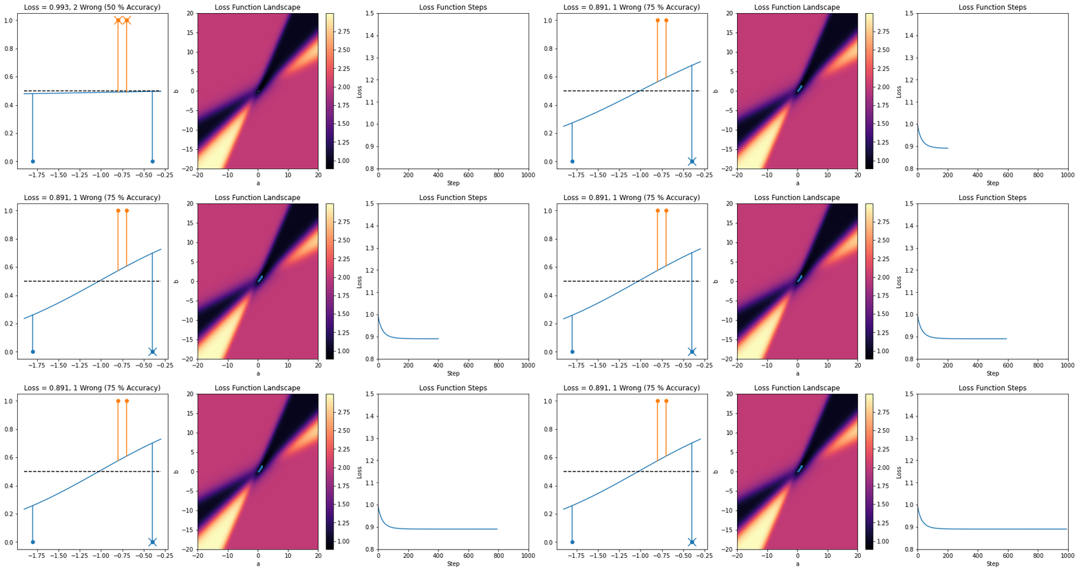
This seems like it worked pretty well on the example we looked at, but there is a theoretical problem. To get at it, let's look at a simpler example where something strange can happen. In particular, let's setup the following data

• 2 points with a 0 label at x=-1.8 and x = -0.4
• 2 points with a 1 label at x=-0.7 and x = -0.8

Let's suppose we take an initial guess of a = 0, b = 0 for our parameters, and then we run gradient descent from that point in parameter space. Here is what we get, which converges nicely to something with a squared loss of 0.891

However, if we start with an initial guess of a = -7, be = -2, we end up converging to a different local min with slightly higher loss

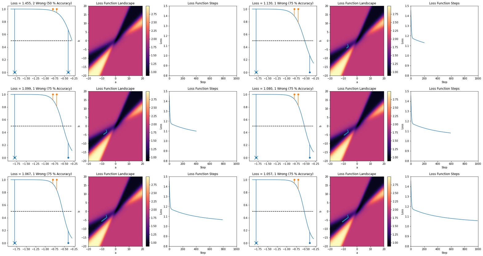
The problem here is that there are additional local mins of squared loss over the parameter space in addition to the global min. If we're unlucky about our initial guess, we may end up in a non-optimal local min that's not a global min. We could try starting at multiple different places and leading to the one which gives the best result, like we did in K-Means clustering task 3, but there is a better answer for logistic regression.

Convexity

The root of the issue for why we can end up with more than one local min is that the loss function we're using is nonconvex. For example, the loss function of the centered logistic function if y = 0 is

which is shown in a plot below

A convex function has the property that a line segment between any pairs of points on the graph of the function stays above the graph. We see that we can violate this with the squared logistic function, as shown by the example below (in which a line segment should always stay in the pink region above the graph if the function is convex)

And the squared loss for y = 1 looks exactly the same but reflected about the y-axis, so it has the same problem.

Let's devise another loss function that is convex, which we'll call logistic loss. We'll start by taking the negative log of the logistic function

Here's what this looks like

We see that this function actually is convex! Also, if we are trying to solve for an input where the logistic function should be closest to 1 (i.e. we're on the positive side of the x-axis), then this loss function makes sense; we get an increasing penalty when we go in the negative direction and a very small penalty when we go in the positive direction.

We can create a very similar loss function for the case when y = 0 as

Which will also be convex (like the squared loss, it is a reflection about the y-axis of the original function -log(f(u))). Below is a plot comparing both squared loss functions

In addition to being convex, these loss functions have a really nice property that they always decrease as we get further away from the target value; that is, they don't suffer from the problem of vanishing gradients like the squared loss, which flattens out on both sides. A vanishing gradient is a terrible thing if we're far on the wrong side, because the derivative may be numerically zero and we'll have no idea what direction we need to walk, but we're actually super far from where we need to be.

Now let's put both of the logistic loss functions together into one final equation for logistic loss over the entire dataset. We'll multiply the 1-loss term by y so that it's only active for y = 1, and we'll multiply the 0-loss term by (1-y) so it's only active for y = 0

Logistic Loss

To show that the above function is convex, we use two properties of convex functions

1. The composition of convex functions is still convex
2. The sum of convex functions is still convex

Our final loss function is the sum of compositions of individual convex functions with "affine functions" (e.g. ax + by + c or ax + by + cz + d), which are completely flat and hence also convex. So the whole thing is convex.

Why do we care so much about convex functions though? It's because they can have at most a single minimum. This means that there's only one place gradient descent can converge to if we choose the step size correctly, so it doesn't matter where the min is with respect to our initial guess.

Taking The Gradient

Now that we know that using the logistic loss is a good idea, let's take its gradient so we can apply gradient descent. Let's suppose we're taking the derivative with respect to some parameter w of which each parameter u_i is a function (such as the parameter a in u_i = ax_i + by_i + c)

which can be simplified to

Which simplifies quite nicely down to

Since we move in the negative direction of the gradient in gradient descent, this translates into the rule

where α is the learning rate. This is a super nice equation, and it's very intuitive! What is says is we need to update a parameter at a rate proportional to the difference between the logistic function and the labels y_i. For instance, if y_i is a 1 and f(y_i) is close to 0, we need to move our parameter w in the positive direction. Conversely, if y_i is a 0 and f(y_i) is close to 1, we need to move w in a negative direction.

To summarize for general high dimensional logistic regression, if

\[ f(\vec{w}, c) = f(\vec{w} \cdot \vec{x}, c) = f( w_1x_1 + w_2x_2 + ... + w_dx_d + c ) \]

Then the update rules are

\[ w_k \gets w_k + \alpha \sum_{i=1}^N x_k(y_i - f(\vec{w}, c)) \]

\[ c \gets c + \alpha \sum_{i=1}^N (y_i - f(\vec{w}, c)) \]

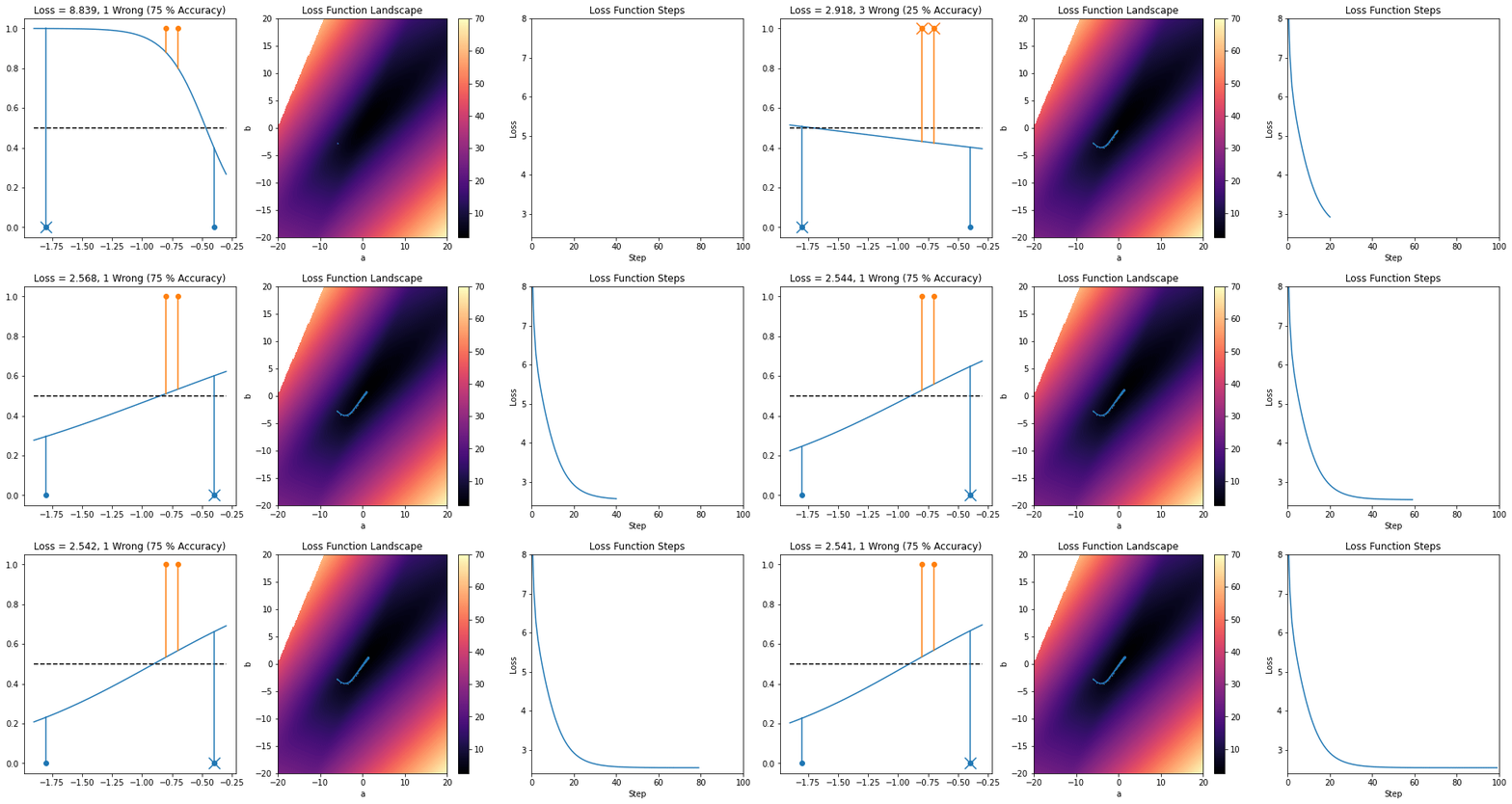
Below is running this on the pathological example we started from the point that ended up with a non-optimal local min with squared loss. As you can see, there's only one global min at the bottom of the hill

Code

The notebook below shows the code I used to generate the pathological example for a squared loss that has more than one local min. You may find some useful tidbits in here for assignment 6.